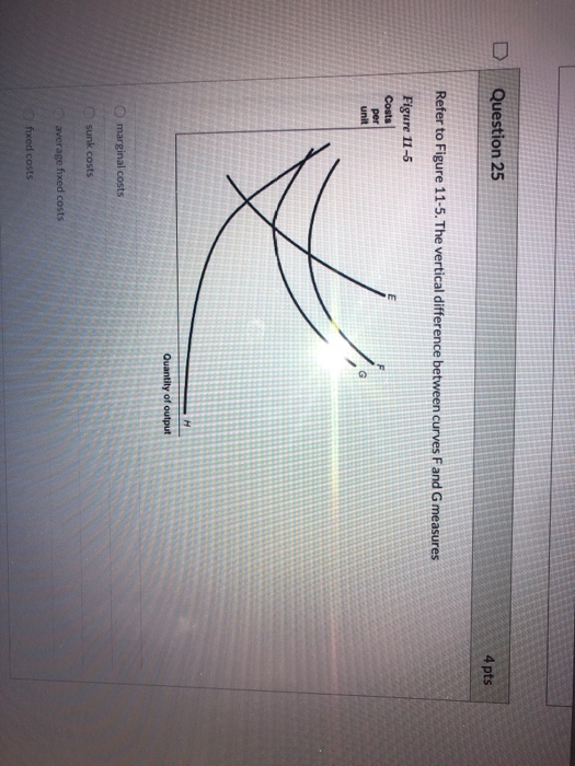
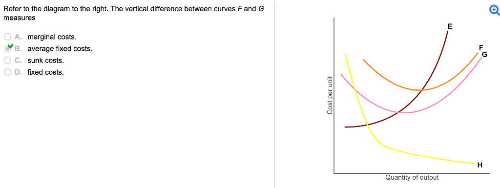
45 refer to the diagram to the right. the vertical difference between curves f and g measures

(210-VI-EFH, October 2008) 1-vii Part 650 Engineering Field Handbook Chapter 1 Surveying Tables Table 1-1 Accuracy standards for horizontal and vertical control 1-3 Table 1-2 List of common abbreviations used 1-12 Table 1-3 Calculations for the angles and sides in figure 1-7 1-19 Table 1-4 Relationships between azimuths and bearings 1-25 the average cost curve and the marginal cost curve to shift downwards. ... Refer to Figure 10-4. The vertical difference between curves F and G measures.

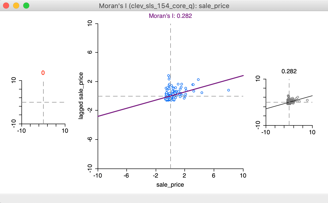
Scatter plots are used to observe relationships between variables. The example scatter plot above shows the diameters and heights for a sample of fictional trees. Each dot represents a single tree; each point's horizontal position indicates that tree's diameter (in centimeters) and the vertical position indicates that tree's height (in ...

Refer to the diagram to the right. the vertical difference between curves f and g measures

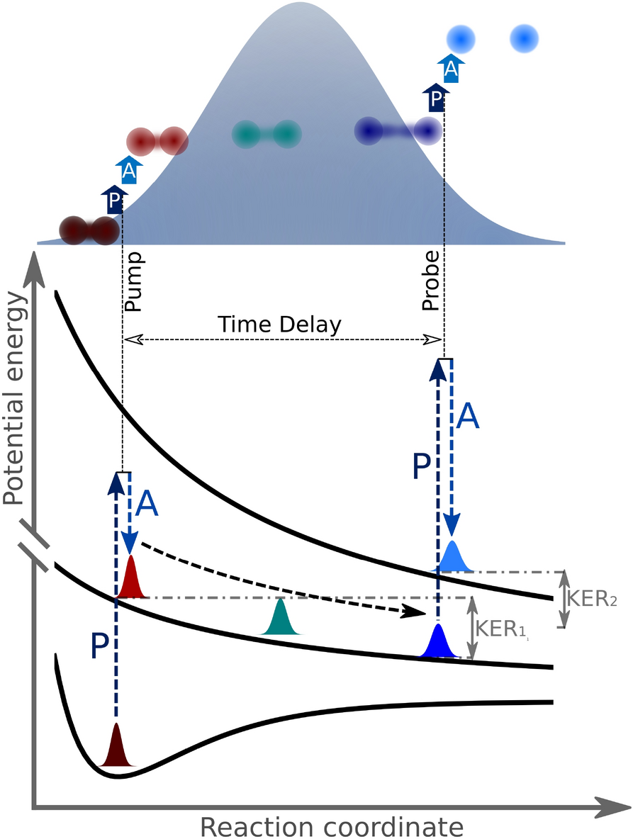
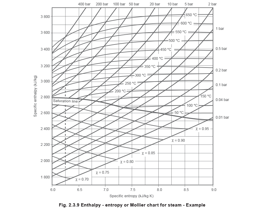
Latent heat can be calculated by use of the diagram in Figure 5. Latent heat is shown by the distance between the saturated liquid line, to the left of the curve, and the saturated vapor line on the right. The difference between the enthalpy of the saturated vapor and that of the saturated liquid is the latent heat of vaporization. The AA-DD model integrates the workings of the money-Forex market and the G&S model into one supermodel. The AA curve is derived from the money-Forex model. The DD curve is derived from the G&S model. The intersection of the AA and DD curves determines the equilibrium values for real GNP and the exchange rate. separation between the PPF and the Budget constraint after Indonesia opens to trade. (e) Draw a world supply schedule which shows rug production relative to cameras. Label all axes, curves, intercepts, and kink points. (f) Add a relative demand schedule to your diagram that implies that Malaysia is incompletely specialized.

Refer to the diagram to the right. the vertical difference between curves f and g measures. Refer to the diagram to the right. The vertical difference between curves F and G measures A. fixed costs. B. sunk costs. C. marginal costs. D. average fixed costs. D. 28. Refer to the table to the right which shows the technology of production at the Matsuko's Mushroom Farm for the month of May. Diminishing marginal returns sets in when the _____ worker is hired. A. 2nd B. 3rd C. 4th D. None ... Refer to the diagram to the right. The vertical difference between curves F and G measures marginal costs. average fixed costs. sunk costs. fixed costs. Question: Refer to the diagram to the right. The vertical difference between curves F and G measures marginal costs. average fixed costs. sunk costs. fixed costs. Using the phase diagram for water given in Figure 2, determine the state of water at the following temperatures and pressures: (a) −10 °C and 50 kPa (b) 25 °C and 90 kPa (c) 50 °C and 40 kPa (d) 80 °C and 5 kPa (e) −10 °C and 0.3 kPa (f) 50 °C and 0.3 kPa. Solution May 25, 2011 SECTION 3.1 Definition of the Derivative 103 In Exercises 11-14, refer to Figure 12. 1 2 3 5 4 123456789 x y FIGURE 12 Graph of f(x). 11. Determine f (a) for a = 1, 2, 4, 7. solution Remember that the value of the derivative of f at x = a can be interpreted as the slope of the line tangent to the graph of y = f(x)at x = a.From Figure 12, we see that the graph of y = f(x)is a ...

Refer to the diagram to the right. The vertical difference between curves F and G measures The vertical difference between curves F and G measures As the size of the firm increases it becomes more difficult to coordinate the operations of its manufacturing plants. 2. Horizontal and Vertical Alignment Relationship 3. Establish Control Points 4. Horizontal Alignment 5. Vertical Alignment 6. Sight Distance 7. Geometric Cross Section a. Pavement Structure b. Profile Grade Location and Cross Slope c. Lane and Shoulder Widths d. Foreslopes e. Roadway Ditches f. Cut and Fill Slopes g. Rock Cut Slopes h ... a linear pair whose vertex is F 62/87,21 Sample answer: A linear pair is a pair of adjacent angles with non common sides that are opposite rays. DQG DUHOLQHDUSDLUZLWKYHUWH[ F, DQG DUHOLQHDUSDLUZLWKYHUWH[ F. an angle complementary to FDG 62/87,21 Complementary angles are two angles with measures that have a sum of 90. Since LVFRPSOHPHQWDU\WR Refer to the diagram to the right. The vertical difference between curve F and G measures. average fixed costs. The marginal product of labor is defined as . the additional output that results when one more worker is hired, holding all other resources constant. If the marginal cost curve is below the average variable cost curve, then. average variable cost is decreasing. Refer to the diagram ...

Refer to Figure 11-5. The vertical difference between curves F and G measures -fixed costs. -average fixed costs. -marginal costs. -sunk costs. the right end. In addition, a 1000-lb upward vertical load acts at the free end of the beam. (1) Derive the shear force and bending moment equations. And (2) draw the shear force and bending moment diagrams. Neglect the weight of the beam. Solution Note that the triangular load has been replaced by is resultant, which is the force 0.5 (12) (360) = 2160 lb (area under the loading diagram ... Refer to the diagram to the right. The vertical difference between curves F and G measures. average fixed costs. Refer to the diagram to the right. Identify the curves in the diagram. E = marginal cost curves, F = average total cost curve, G = average variable cost curve, H= average fixed cost curve. Refer to the diagram to the right. Diminishing marginal productivity sets in after . the 2nd ... Academia.edu is a platform for academics to share research papers.

then the indifference curves would be vertical and utility is increasing to the right as more beer is consumed. b. Betty is indifferent between bundles of either three beers or two hamburgers. Her preferences do not change as she consumes any more of either food. Since Betty is indifferent between three beers and two burgers, an indifference curve

Refer to Figure 11-5. The vertical difference between curves F and G measures a) average fixed costs. b)fixed costs. c)marginal costs. d)sunk costs.

Refer to the diagram to the right the vertical difference between curves f and g measures. B intersects the horizontal axis at a point corresponding to the 5th worker. In a diagram that shows the marginal product of labor on the vertical axis and labor on the horizontal axis the marginal product curve 10 a never intersects the horizontal axis.

b. supply curve downward (or to the right). c. demand curve upward (or to the right). d. demand curve downward (or to the left). ____ 25. When a tax is imposed on a good for which demand is elastic and supply is elastic, a. sellers effectively pay the majority of the tax. b. buyers effectively pay the majority of the tax.

Identify the curves in the diagram. E = marginal cost curve; F = average total cost curve; G = average variable cost curve; H = average fixed cost curve. ... Refer to Figure 11-5. The vertical difference between curves F and G measures. average fixed costs. 1. If average total cost is $50 and average fixed cost is $15 when output is 20 units ...

4.1.1 Recognize a function of two variables and identify its domain and range. 4.1.2 Sketch a graph of a function of two variables. 4.1.3 Sketch several traces or level curves of a function of two variables. 4.1.4 Recognize a function of three or more variables and identify its level surfaces. Our first step is to explain what a function of ...

Iso-Product Curves Slope Downward from Left to Right: ... LM, and NP segments of the elliptical curves are the isoquants. Difference between Indifference Curve and Iso-Quant Curve: The main points of difference between indifference curve and Iso-quant curve are explained below: 1. Iso-quant curve expresses the quantity of output. Each curve refers to given quantity of output while an ...

21) Refer to Figure 11 -5. The vertical difference between curves F and G measures 21) A) marginal costs. B) fixed costs. C) average fixed costs. D) sunk costs. 22) Refer to Figure 11 -5. Curve G approaches curve F because 22) A) fixed cost falls as capacity rises. B) total cost falls as more and more is produced.

The vertical difference between curves F and G measures. average fixed costs. Image: Refer to the diagram to the right. The vertical difference between ...

Label area between MAC1 and MAC2 to the right of e1 as a. Label area below MAC2 to the right of e1 as b. Label area bounded by the charge line, MAC2, and e1 line as d. Label area bounded by MAC2, e1 line, and e2 line as c. Label area bounded by the charge line, e2 line, and the two axes as f. Compliance cost with MAC1 technology = (a+b+c+d+f)

The first curve shows a strong acid being titrated by a strong base. There is the initial slow rise in pH until the reaction nears the point where just enough base is added to neutralize all the initial acid. This point is called the equivalence point. For a strong acid/base reaction, this occurs at pH = 7.

They run horizontally from left to right and are labeled on the left side of the diagram. Pressure is given in increments of 100 mb and ranges from 1050 to 100 mb. Notice the spacing between isobars increases in the vertical (thus the name Log P).

The vertical distance between the original and new supply curve is the amount of the tax. Due to the tax, the new equilibrium price (P1) is higher and the equilibrium quantity (Q1) is lower. While the consumer is now paying price (P1) the producer only receives price (P2) after paying the tax.

P.C.C. Point of compound curvature - Point common to two curves in the same direction with different radii P.R.C. Point of reverse curve - Point common to two curves in opposite directions and with the same or different radii L Total length of any circular curve measured along its arc Lc Length between any two points on a circular curve

The composite of two functions f and g, written f g, is: f g( x ) = f ( g( x )) The domain of the composite function f g( x ) = f ( g( x )) consists of those x-values for which g( x ) and f ( g( x )) are both defined: we can evaluate the composition of two functions at a point x only if each step in the composition is defined.

Appendix B: Indifference Curves Economists use a vocabulary of maximizing utility to describe people's preferences. In Consumer Choices, the level of utility that a person receives is described in numerical terms. This appendix presents an alternative approach to describing personal preferences, called indifference curves, which avoids any need for using numbers to measure utility.

separation between the PPF and the Budget constraint after Indonesia opens to trade. (e) Draw a world supply schedule which shows rug production relative to cameras. Label all axes, curves, intercepts, and kink points. (f) Add a relative demand schedule to your diagram that implies that Malaysia is incompletely specialized.

The AA-DD model integrates the workings of the money-Forex market and the G&S model into one supermodel. The AA curve is derived from the money-Forex model. The DD curve is derived from the G&S model. The intersection of the AA and DD curves determines the equilibrium values for real GNP and the exchange rate.