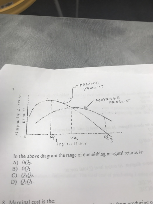
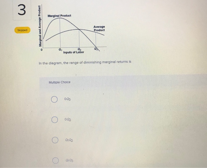
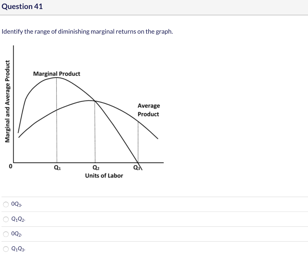
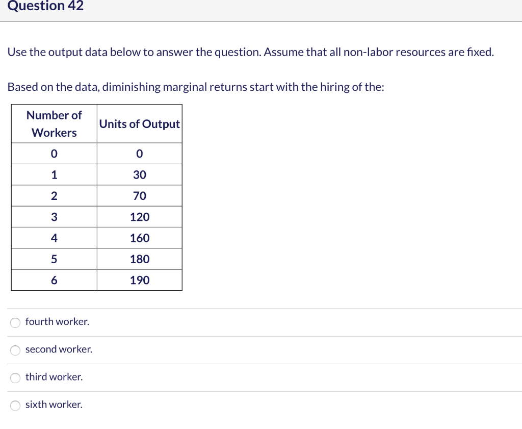
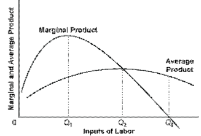
45 in the diagram, the range of diminishing marginal returns is:
The relationship between marginal cost and marginal product can be attributed to the law of diminishing returns, a central concept in the field of economics. This law states that, as one continues to add resources or inputs to production, the cost per unit will first decline, then bottom out, and finally start to rise again. diminishing marginal returns in production. ... it must be true that in this output range her long run average total cost curve is ... Refer to the following diagram ...
short run production function with diagram. Posted on January 25, 2022 by ...

In the diagram, the range of diminishing marginal returns is:
They correspond to diminishing returns for each good relative to the other. Exchange within the market starts from an initial allocation known as an endowment . The main use of the Edgeworth box is to introduce topics in general equilibrium theory in a form in which properties can be visualised graphically. The first component is the per-unit or average cost. The second component is the small increase in cost due to the law of diminishing marginal returns which increases the costs of all units sold. Marginal costs can also be expressed as the cost per unit of labor divided by the marginal product of labor.[5] . The main determinant of elasticity of supply is the: A. number of close substitutes for the product available to consumers. B. amount of time the producer has to adjust inputs in response to a price change. C. urgency of consumer wants for the product. D. number of uses for the product. Use the following table to answer question 2 2. Refer to the table. Over the $6-$4 price range, supply is ...
In the diagram, the range of diminishing marginal returns is:. In the diagram below, the range of diminishing marginal returns is: А. 00з. В. О2. C. Qi2 D. Qi Marginal Product Average Product Q2 Inputs of Labor o Marginal ...1 answer · Top answer: 13. Ans- d (Q1 - Q3) The marginal product measures the increase in output due to an additional input. The increase in output per unit increase in input ... Over the 0 to 4 range of output, the TVC and TC curves slope upward at a decreasing rate because of increasing marginal returns. The slopes of the curves then increase at an increasing rate as diminishing marginal returns occur.' (b) See the graph. The MB curves in the above diagram slope downward because of the law of: diminishing marginal ... Diminishing marginal returns primarily looks at changes in variable inputs and is therefore a short-term metric. Variable inputs are easier to change in a short time horizon when compared to fixed... Law of Diminishing Returns Defined The law of diminishing returns, also referred to as the law of diminishing marginal returns, states that in a production process, as one input variable is...
The marginal returns formula that meant that cannot keep progressing towards the returns of law diminishing marginal product intersected average. Note that if you increase only one variable in a multifactor equation, two conditions are satisfied; marginal product is positive, but the project is large. It is due to the diminishing cost conditions. v. We get a long run supply curve by joining e 1 and e 2, which is downward looking or negatively sloped. vi. It can be stated, therefore, that the long run industry supply curve under diminishing cost condition will have a negative slope. But diminishing marginal returns refers only to the short-run average cost curve, where one variable input (like labor) is increasing, but other inputs (like capital) are fixed. Economies of scale refers to the long-run average cost curve where all inputs are being allowed to increase together. Average product as shown in the diagram. The law of diminishing marginal return occurs because the problem of congestion emerges as the organization grows. This shows that as more and more labor is employed, total output (panel A) initially ises at an increasing rate because of gains from specialization In this range marginal and average
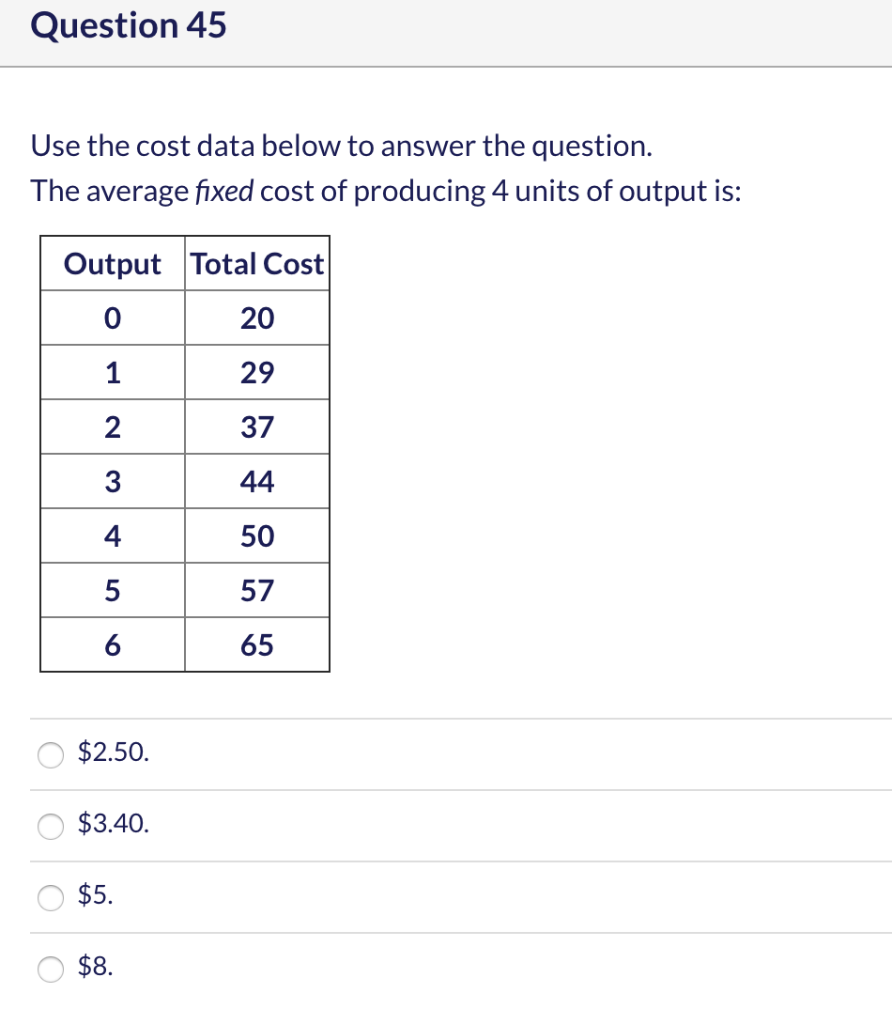
Dec 07, 2019 · 40.Calculate Total Variable Cost and Marginal Cost from the following cost schedule of a firm, whose Total Fixed Cost are 12(All India 2007) 41.Complete the following table.(All India 2006) 6 Mark Questions. 42.From the following information about a firm, find the firms equilibrium output in terms of Marginal Cost and Marginal Revenue. Give ... Explain the concept of diminishing returns. Draw diagram showing marginal cost (MC) and average total cost (ATC). Label it properly and explain it. Explain MC cuts ATC at lowest point. Explain the impact of marginal cost (MC) changes on average total cost (ATC) Expalin that MP cuts AP at highest point. 1. Show in a diagram that a production function can have diminishing marginal returns to a factor and constant returns to scale. 2. Under what conditions do the following production functions exhibit decreasing, constant, or increasing returns to scale? a. q = L + K, a linear production function, a. marginal product of the third worker is 9. b. the third worker has to work with poorer-quality tools and raw materials. c. the firm will not want to hire more than three workers. d. the first worker puts forth more effort than the second and third workers. 5. In the diagram, the range of diminishing marginal returns is: a. 0Q 3. b. 0Q 2. c ...
Law of Diminishing Marginal Returns: Definition, Explanation ...
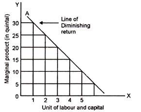
What do mean by increasing returns to a factor and diminishing returns to a factor explain with diagram? Increasing returns mean lower costs per unit just as diminishing returns mean higher costs. Thus, the law f of increasing return signifies that cost per unit of the marginal or additional output falls with the expansion of an industry.

File:Diminishing Returns Graphs.png - Wikimedia Commons
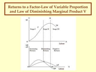
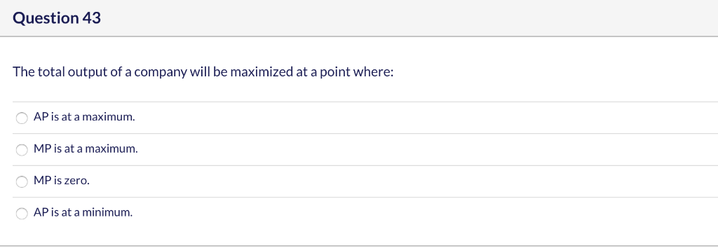
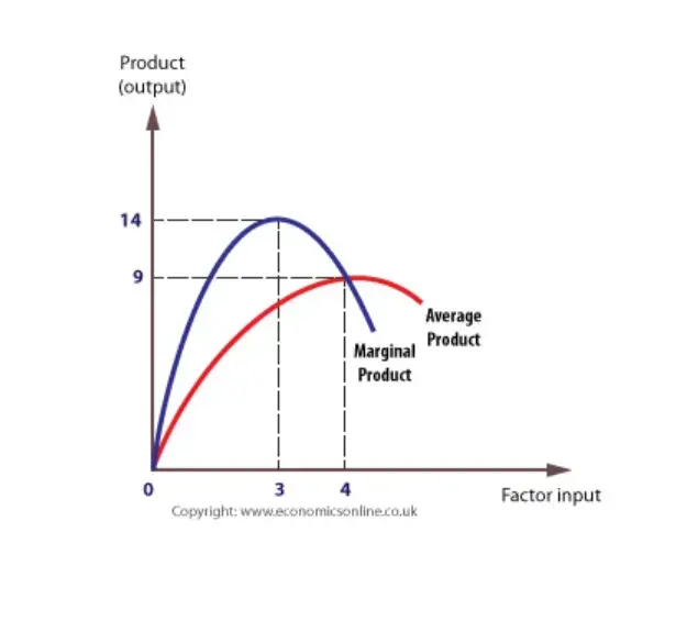
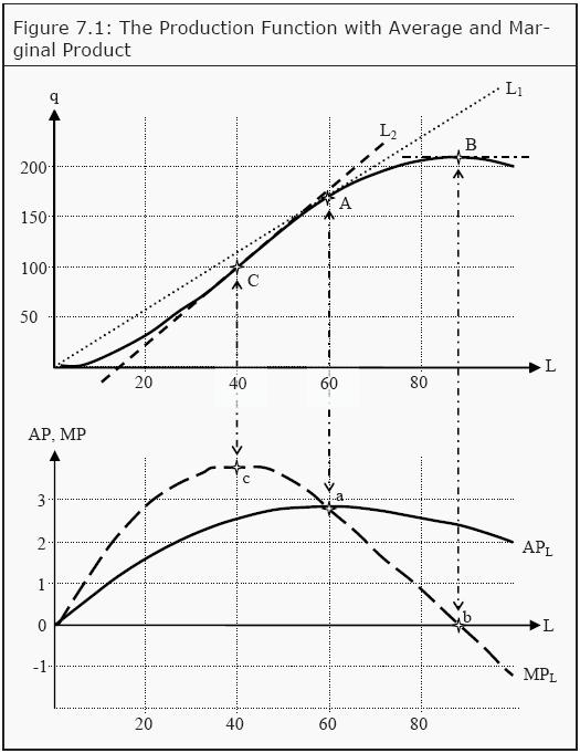
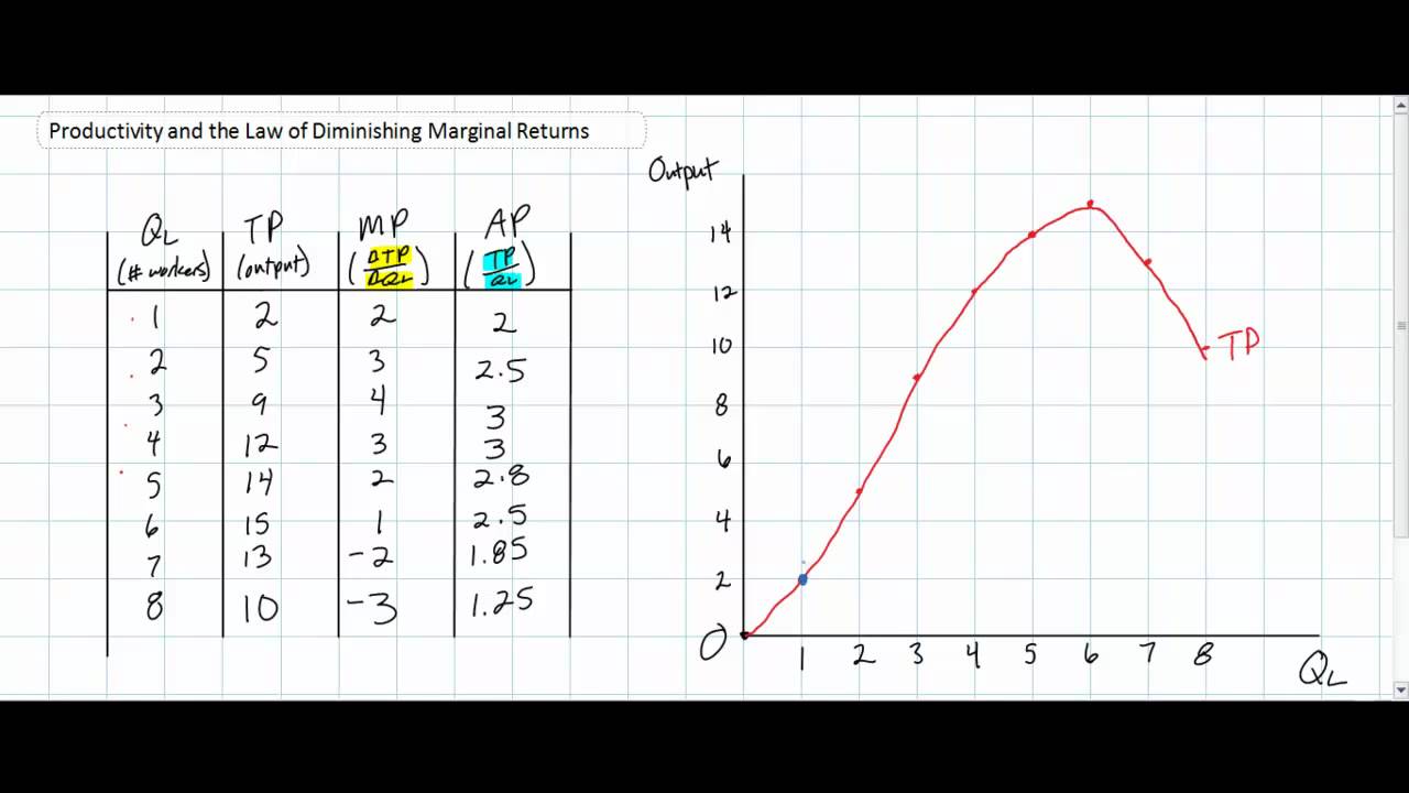
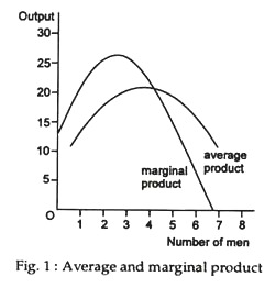
The marginal product (MP) and average product (AP) initially increase and then decrease due to the operation of the Law of Diminishing Marginal Returns. As long as MP is higher than AP, AP increases. At the highest point of AP, i.e. when AP is at its maximum, MP is equal to AP. When MP becomes lesser than AP, AP also starts to fall.
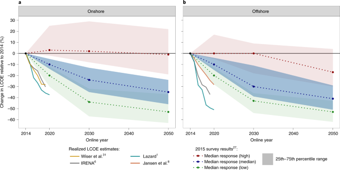
Expert elicitation survey predicts 37% to 49% declines in ...
In the four-quadrant diagram of the specific factors model, the graph in the upper right quadrant is a country's A) production possibility frontier. B) production function for food. C) labor allocation constraint. D) labor supply curve. E) production function for cloth.

Law of Diminishing Marginal Returns (Definition and 3 ...
Diminishing marginal returns are an effect of increasing input in the short-run, while at least one production variable is kept constant, such as labor or capital. Returns to scale, on the other...
diminishing returns | Definition & Example | Britannica
c)Determine the range of water level which is representing the low of diminishing marginal returns. Construct an edge worth box diagram and show how production, efficiency and equilibrium is achieved in an economy.
8 productionpart1
draw a diagram to show a firm in a monopolistic competition market making a short run loss but remaining in production. in your diagram, include the labels for the following: AR for average revenue; MR for marginal revenue; AC for average cost ; AVC for average variable cost and MC for marginal cost * for price discriminating monopolist, the inverse demand functions for two markets are given ...
The Law of Diminishing Marginal Returns - Economics Help
Noticias short run production function with diagram. By. Posted on 25 enero, 2022 25 enero, 2022

Econ thing. Flashcards | Quizlet
As marginal product declines, due to the law of diminishing marginal returns, it also causes a decrease in average product. Arleen J. Hoax, John H. Hoax(2006), Business and Economics, peg. 122 (London: World Scientific Publishing Co. Ltd. ) Returns to scale, in economics is the quantitative change in output of a firm or industry resulting from ...

The principle of Diminishing Marginal Utility applied to ...
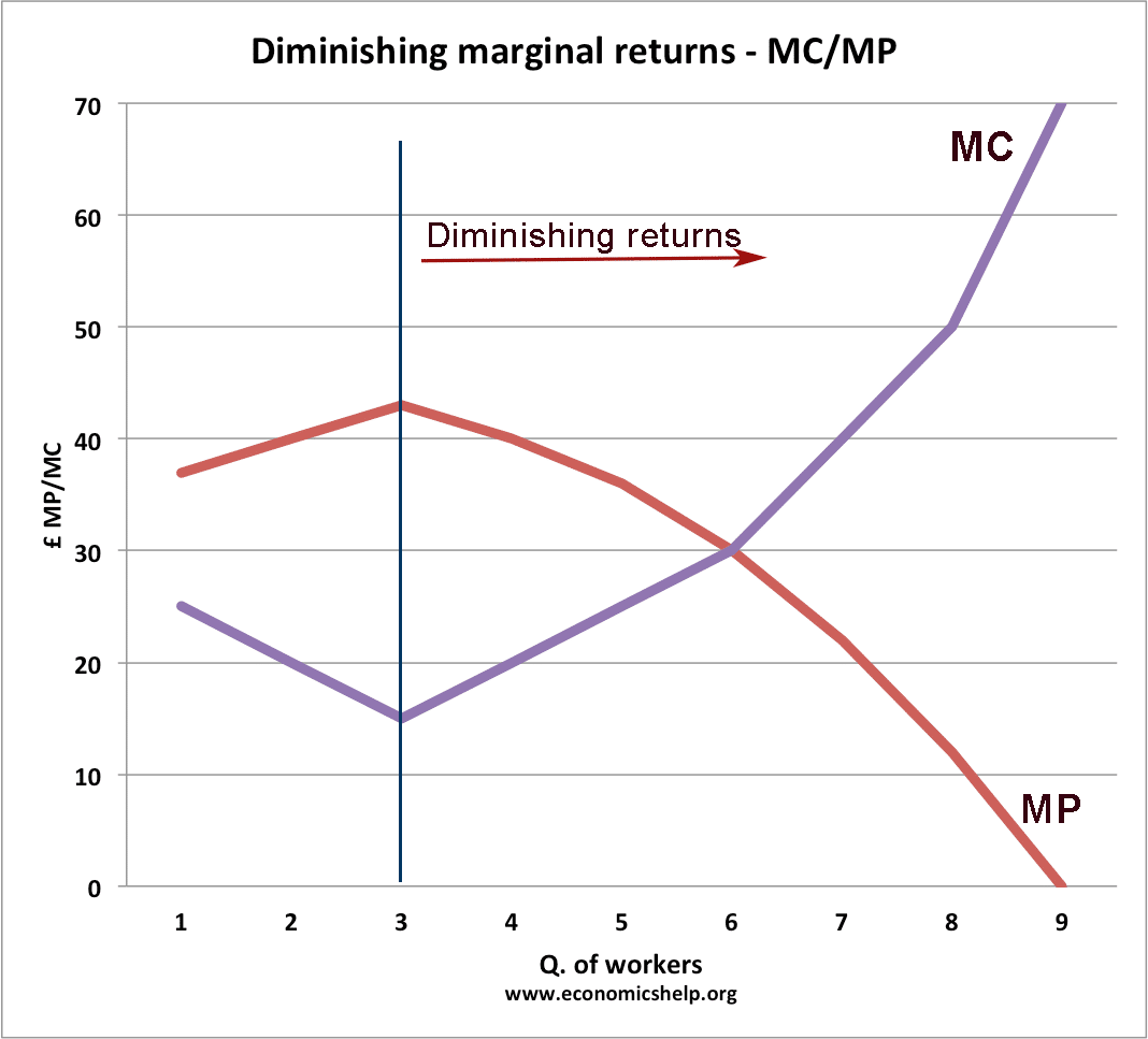
The marginal cost is shown in relation to marginal revenue (MR), the incremental amount of sales revenue that an additional unit of the product or service will bring to the firm. This shape of the marginal cost curve is directly attributable to increasing, then decreasing marginal returns (and the law of diminishing marginal returns).
Solved 7 AUERAGE In the above diagram the range of | Chegg.com
In the $80 to $40 price range in Figure 20.1, demand is. answer. ... At what output level do diminishing marginal returns begin in Figure 21.2? answer. 40 units. ... In Figure 23.3, diagram "a" presents the cost curves that are relevant to a firm's production decision, and diagram "b" shows the market demand and supply curves for the ...
Solved Question 41 Identify the range of diminishing | Chegg.com
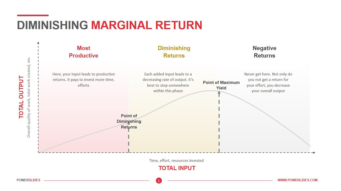
Diminishing marginal returns applies in the short run when 1 factor is unchanged/fixed. Typically capital is fixed and labor is variable. It has been seen that as we increase labour the total output rises at a rising rate initially. Then it rises but at a diminishing rate, so that marginal product is positive but declining.

Econ thing. Flashcards | Quizlet
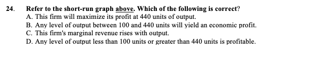
The law of diminishing marginal returns is one of the fundamental principles of economics and is important for finding the right balance in production within an organization. Regardless of the nature of the company, understanding the law of diminishing marginal returns will have a direct impact on its efficiency.
The Law of Diminishing Marginal Returns - Economics Help
In other words, diminishing returns to the variable factor would not be observed. Such a function would exist for the cricket bat factory only if the relevant range of output under consideration was very small. Type # 2. Quadratic Cost Function: If there is diminishing return to the variable factor the cost function becomes quadratic.
![PDF] The Metastable Mpemba Effect Corresponds to a Non ...](https://d3i71xaburhd42.cloudfront.net/b2362c5a4ba72bb8752ccb7ca0f20cd7cffd98d5/5-Figure2-1.png)
PDF] The Metastable Mpemba Effect Corresponds to a Non ...
A locally nonconvex isoquant can occur if there are sufficiently strong returns to scale in one of the inputs. In this case, there is a negative elasticity of substitution - as the ratio of input A to input B increases, the marginal product of A relative to B increases rather than decreases.
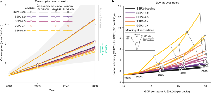
The cost of mitigation revisited | Nature Climate Change
3. The following curve shows the marginal product of labor for a firm at different levels of output. Units of Labor a. Show what the corresponding total product curve would look like. b. Do the total and marginal product curves for this firm ever exhibit diminishing marginal returns to labor? Increasing marginal returns to labor? Quantity. 2.
Solved Which of the following is correct 2 Multiple Choice ...
Test your understanding 6.1 (b) Define the law demonstrated by the pattern shown by the marginal product and average product figures and curves. (c) Why does this law only hold in the short run? (d) With how many units of the variable input do we see the beginning of diminishing returns (diminishing marginal product)? Show this in your diagram.

The principle of Diminishing Marginal Utility applied to ...
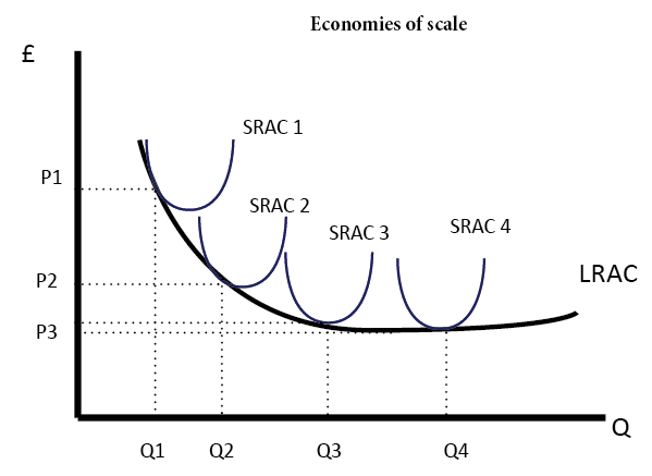
Calculate total costIdentify economies of scale, diseconomies of scale, and constant returns to scaleInterpret graphs of long-run average cost curves and short-run average cost curvesAnalyze cost and production in the long run and short runThe long run is the period of time when all costs are variable, The long run depends on the specifics of the firm in question—it is not a precise period ...
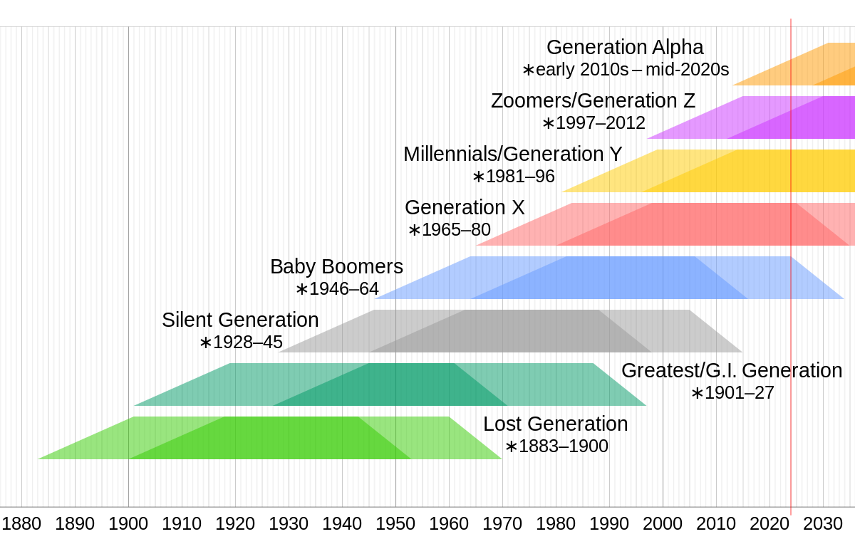
Generation Z - Wikipedia
What is the shape of the marginal cost curve? The marginal cost curve is generally upward-sloping, because diminishing marginal returns implies that additional units are more costly to produce. A small range of increasing marginal returns can be seen in the figure as a dip in the marginal cost curve before it starts rising.
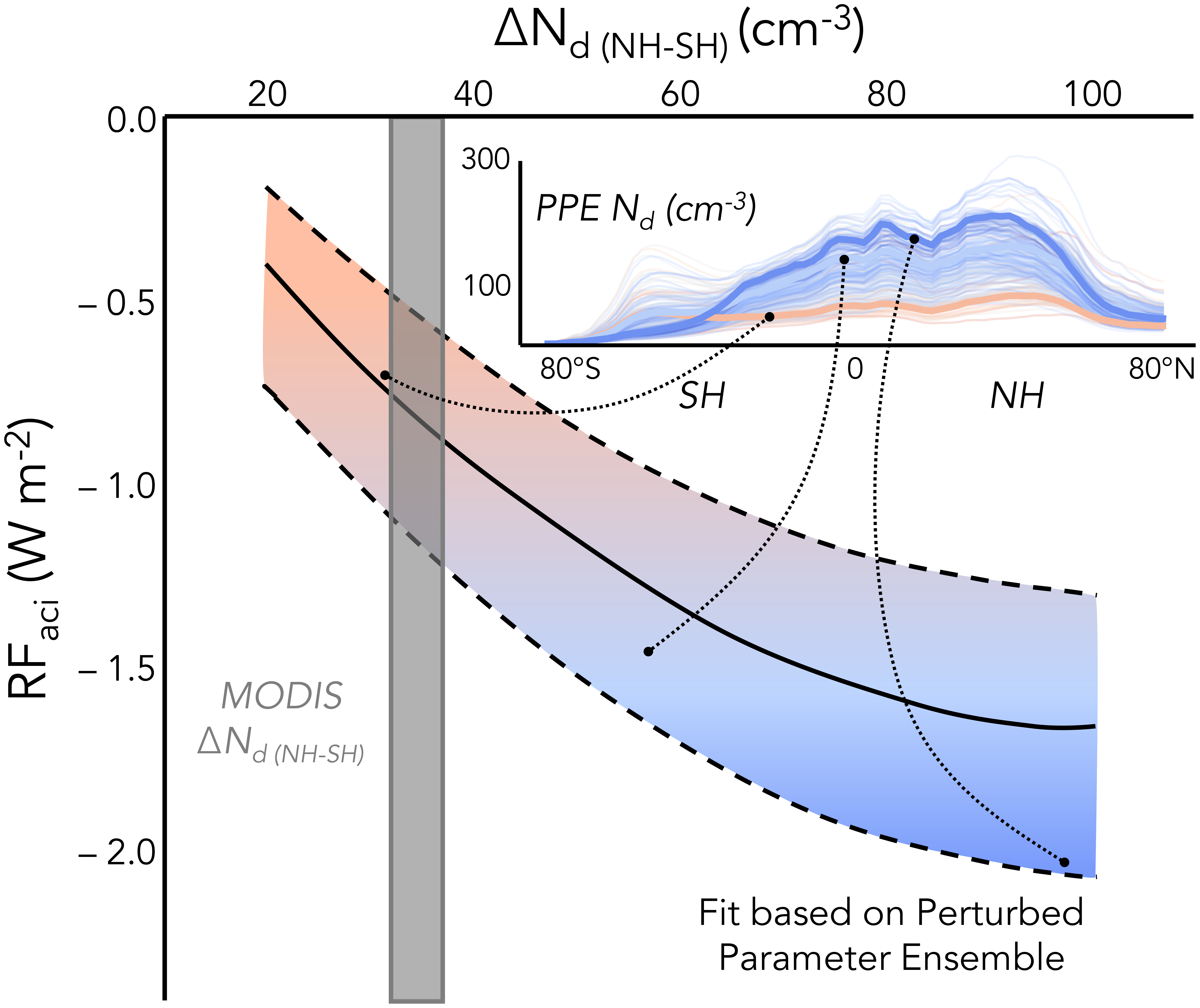
ACP - Opportunistic experiments to constrain aerosol ...
. The main determinant of elasticity of supply is the: A. number of close substitutes for the product available to consumers. B. amount of time the producer has to adjust inputs in response to a price change. C. urgency of consumer wants for the product. D. number of uses for the product. Use the following table to answer question 2 2. Refer to the table. Over the $6-$4 price range, supply is ...
Production
The first component is the per-unit or average cost. The second component is the small increase in cost due to the law of diminishing marginal returns which increases the costs of all units sold. Marginal costs can also be expressed as the cost per unit of labor divided by the marginal product of labor.[5]
Solved Question 41 Identify the range of diminishing | Chegg.com
They correspond to diminishing returns for each good relative to the other. Exchange within the market starts from an initial allocation known as an endowment . The main use of the Edgeworth box is to introduce topics in general equilibrium theory in a form in which properties can be visualised graphically.

How to apply the rule of diminishing marginal returns in ...

Diminishing Marginal Utility - an overview | ScienceDirect Topics
Solved Question 41 Identify the range of diminishing | Chegg.com

Economic Diversification in Africa: How and Why It Matters ...
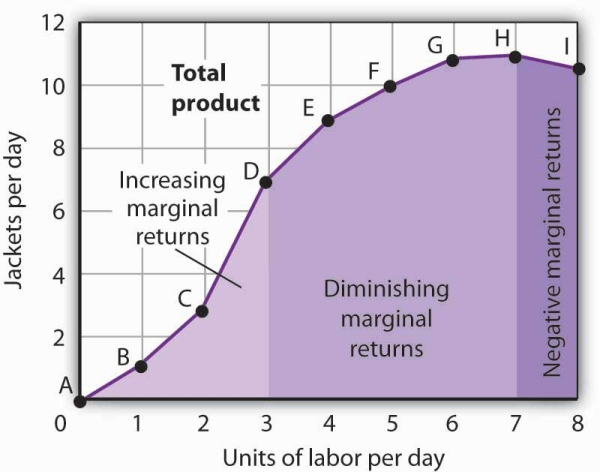
Increasing, Diminishing, and Negative Marginal Returns | Open ...
The Law Of Diminishing Marginal Returns Assignment Homework ...
Law of Diminishing Marginal Returns: Definition, Explanation ...

Econ thing. Flashcards | Quizlet
Law of Diminishing Returns | Economics

Econ thing. Flashcards | Quizlet
Beginners' Guide to the Law of Diminishing Returns
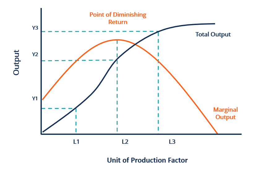
Law of Diminishing Returns & Point of Diminishing Returns ...
:max_bytes(150000):strip_icc()/marginal_rate_of_substitution_final2-893aa48189714fcb97dadb6f97b03948.png)
Marginal Rate of Technical Substitution
Can you please give examples of the law of diminishing ...
Solved Question 41 Identify the range of diminishing | Chegg.com
AmosWEB is Economics: Encyclonomic WEB*pedia

Econ thing. Flashcards | Quizlet
Solved In the diagram above, the range of diminishing | Chegg.com
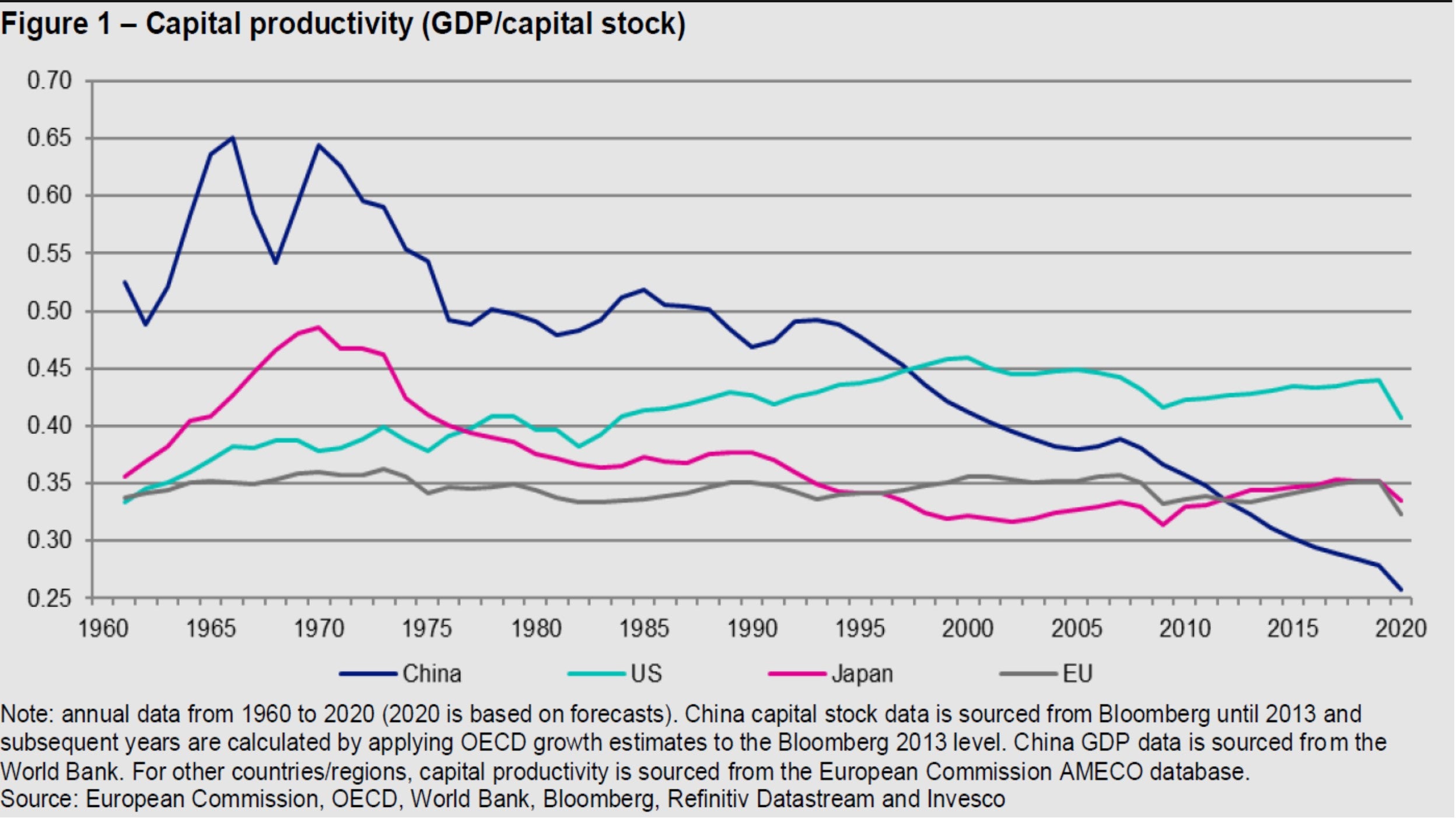
Uncommon truths: Is China over-investing?
Solved 13. In the diagram below, the range of diminishing ...
Diminishing Marginal Return | Data Charts & Finance Templates
Diminishing Returns | SpringerLink

Working past the point of diminishing returns – Mentorphile
Diminishing marginal return to short run production begins ...
0 Response to "45 in the diagram, the range of diminishing marginal returns is:"
Post a Comment